Human contributions to global soundscapes are less predictable than the acoustic rhythms of wildlife

Abstract

Across the world, human (anthropophonic) sounds add to sounds of biological (biophonic) and geophysical (geophonic) origin, with human contributions including both speech and technophony (sounds of technological devices). To characterize society's contribution to the global soundscapes, we used passive acoustic recorders at 139 sites across 6 continents, sampling both urban green spaces and nearby pristine sites continuously for 3 years in a paired design. Recordings were characterized by bird species richness and by 14 complementary acoustic indices. By relating each index to seasonal, diurnal, climatic and anthropogenic factors, we show here that latitude, time of day and day of year each predict a substantial proportion of variation in key metrics of biophony—whereas anthropophony (speech and traffic) show less predictable patterns. Compared to pristine sites, the soundscape of urban green spaces is more dominated by technophony and less diverse in terms of acoustic energy across frequencies and time steps, with less instances of quiet. We conclude that the global soundscape is formed from a highly predictable rhythm in biophony, with added noise from geophony and anthropophony. At urban sites, animals experience an increasingly noisy background of sound, which poses challenges to efficient communication.

Check the full text

Somervuo, P., Roslin, T., Fisher, B. L., Hardwick, B., Kerdraon, D., Raharinjanahary, D., ... & Mata, V. A. (2025). Human contributions to global soundscapes are less predictable than the acoustic rhythms of wildlife. Nature ecology & evolution, 1-14.

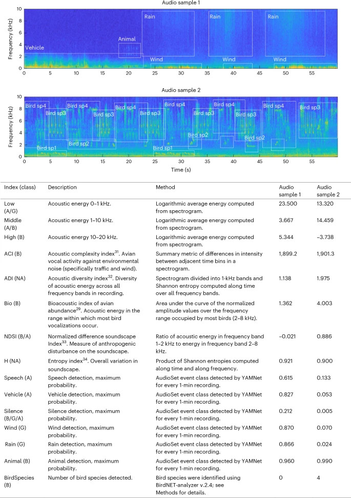
Fig. 1: Acoustic indices used to track the rhythms in the global soundscape. Top: two example spectrograms with the signatures of different sound sources highlighted and identified. Bottom: table lists and briefly defines 15 acoustic indices of the soundscape. In the table and in all subsequent figures, we sort indices by their type (how they are calculated), whereas letters clarify how they are assigned: B, biophony; G, geophony; A, anthropophony; or NA, no clear classification. The values of each index for the example audio clips are given in the last two columns. sp, species.

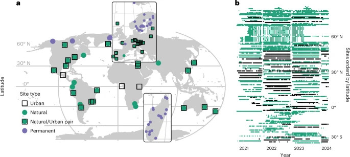
Fig. 2: Sampling design and coverage. a, Across the world, we used up to five AudioMoth31 samplers to record the local soundscape at each of 139 sites. To characterize differences between natural sites (filled green circles) and urban green spaces (open black squares), 83 of the sites were part of a paired design, with each habitat type sampled for a year within a distance of 4–50 km. To avoid the effects of specific years, the starting habitat (natural or urban green space) was randomized between sites. For part of the material (violet symbols), the habitat was fixed to natural sites alone. b, This resulted in multi-annual time series for individual sites (y axis), with the coverage of individual weeks shown by squares across time on the x axis. Habitats are coloured green for natural and black for urban green space.

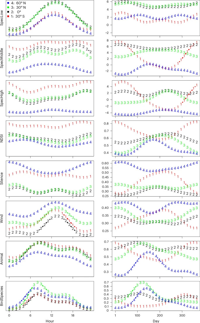
Fig. 3: Seasonal and diurnal variation in different acoustic indices. Predictions for the hour of the day (left) and day of the year (right) for 30° S, 0°, 30° N and 60° N. The predictions shown are based on the global model fitted to all data and shown for those eight indices for which the seasonal and diurnal patterns explained a substantial part of the variation (Fig. 4). Here time is represented by local absolute time; for patterns with respect to time relative to sun time, see Supplementary Fig. 57. Site-specific results for all acoustic indices are shown in Supplementary Information 1. For definitions of each index, see Fig. 1.

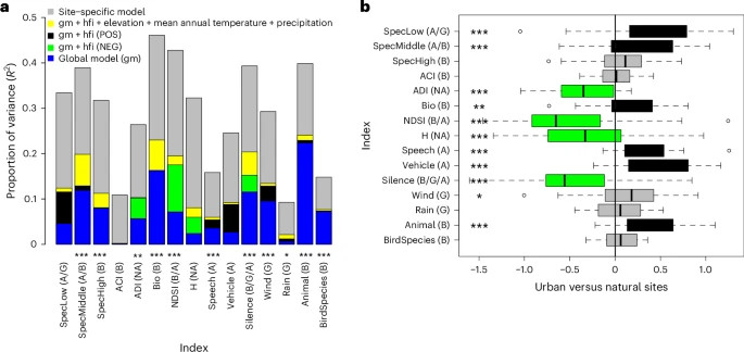
Fig. 4: Predictability of 15 acoustic indices in space and time and differences across pairs of natural versus urban sites. a, Predictability of 15 acoustic indices in space and time. The total height of each bar shows the proportion of variance explained (R2) by site-specific models. The blue section shows variation explained by the latitude of the site using a global model (gm). The significance of latitude was determined by a permutation test (two-sided; 139 sites; 1,000 permutations; no adjustment for multiple comparisons), with index-specific P values as follows: 0.733, 0.001, 0.001, 0.693, 0.003, 0.001, 0.001, 0.359, 0.001, 0.106, 0.001, 0.001, 0.018, 0.001 and 0.001. Significance levels are *P ≤ 0.05, **P ≤ 0.01 and ***P ≤ 0.001. Black (positive effect, POS) and green (negative effect, NEG) sections show the increase in R2 with the addition of the site-specific human footprint index (hfi) to the global model. The yellow sections indicate the increase in R2 when climatic conditions (elevation, mean annual temperature and precipitation) are added to a model including hfi. b, Differences observed across pairs of natural versus urban sites. Each box shows the distribution of empirically observed pairwise differences between the two sites within a pair—with a box for the interquartile range (50% of data), a vertical line for the median; whiskers for the minimum and maximum up to 1.5× interquartile range from the box; and individual data points for outliers beyond this range. Since the difference is calculated as urban minus natural values, a positive value indicates higher values for urban sites (significant differences shown by black boxes) whereas a negative value indicates higher values at natural sites (significant differences shown by green boxes). Index-specific P values from two-sided t-tests across 36 paired values (without adjustments for multiple comparisons): 1.06 × 10−5, 7.91 × 10−4, 1.46 × 10−1, 8.60 × 10−1, 1.89 × 10−7, 3.06 × 10−3, 2.45 × 10−5, 5.71 × 10−4, 9.51 × 10−9, 3.46 × 10−8, 5.41 × 10−6, 2.65 × 10−2, 3.27 × 10−1, 1.10 × 10−6 and 6.07 × 10−2 (with asterisks as in a). Index letters as in Fig. 1. Diel variation was modelled by local absolute time; for patterns with respect to sun time, see Supplementary Fig. 58.

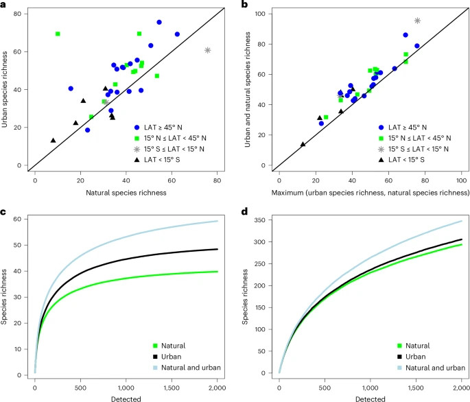
Fig. 5: Species richness for 36 site pairs composed of natural and urban sites. a,b, Species richness for individual urban and natural sites addressing whether urban or natural sites have more species (a) and whether urban and natural sites have different species (b). c,d, Species richness as a function of the number of bird detections sampled separately for each site after which we averaged the resulting curves (c) and in samples from pooled natural and pooled urban sites (d). Green curves emanate from natural sites and black curves from urban green spaces. Light-blue curves are based on data combined across the natural site and its paired urban green space, and thereby represent sampling of recordings irrespective of the environment of origin. The data include bird detections (BirdNET confidence threshold 0.8) for which recordings were available for both urban and natural sites at the same day of the year and the same time of the day within each pair. The resulting data have been sampled with replacement. In a and b, species richness S is defined as the number of distinct species in 1,000 detections, whereas c and d show the accumulation of species richness detected up to 2,000 detections. All results are averages across 50 replicates. LAT, latitude.